
1.3: Maps and Graphs
Create and interpret maps and graphs.
The next geography tool we want to put into your toolbox is that of creating and interpreting maps and graphs. Maps and graphs provide visual representations of otherwise abstract data. You will be creating and using them throughout this course, as well as encountering them throughout your lifetime.
Making maps is something most students have done since they were very young. Perhaps you started off by drawing a map of your room or the rooms of your house. Maybe you made a map of your school and the playground. You have probably created a map of your state and its major geographical features. As we study geography, we need the ability to create both mental maps and picture maps. A mental map is what we use when we are thinking about how to get someplace. For instance, imagine going to the nearest grocery store. Do you know which direction to go and where to turn? If you can get from one place to another in your mind, then you are creating a mental map. Creating a mental map enables you to give directions or even sketch out a map for someone else to follow.
Maps are created for many different reasons. Often data is added to maps in order to provide a clear picture of various features. In this segment of the lesson you will learn to use data to add features to maps. In this case you will add colors to a map in order to signify variations in population density, creating a population map. You will then use the information from the map to create a graph that accurately reflects population information.
I will demonstrate the process for you, and then you will have a chance to do it yourself. We will start with an outline map of Arizona and its counties.
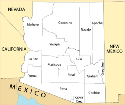
Figure 1.3.1, An outline map of Arizona and its counties. (“Arizona County Map,” National Atlas of the United States, 2004. http://nationalatlas.gov/printable /reference.html#list)
© BYU Independent Study
Now I will add color to the counties based on the data collected on population, and I will create a legend to explain what the colors indicate. Here is the data that I will use to decide what color each county should be colored.
|
County |
Population/sq. mile |
County |
Population/sq. mile |
|---|---|---|---|
|
Apache |
4–12 |
Mohave |
4–12 |
|
Cochise |
13–28 |
Navajo |
4–12 |
|
Coconino |
4–12 |
Pima |
34–92 |
|
Gila |
4–12 |
Pinal |
29–33 |
|
Graham |
4–12 |
Santa Cruz |
29–33 |
|
Greenlee |
4–12 |
Yavapai |
13–28 |
|
La Paz |
4–12 |
Yuma |
29–33 |
|
Maricopa |
93–334 |
||
|
Information found on http://factfinder.census.gov. |
|||
I must make the legend before I color the map. I then use the legend and the data list to guide me as I color the map.
These are the colors that I will use to indicate population density:
| Color | Population/sq. mile |
|---|---|
|
Yellow |
4–12 |
|
Orange |
13–28 |
|
Purple |
29–33 |
|
Red |
34–92 |
|
Green |
93–334 |
Here is the color-coded map.
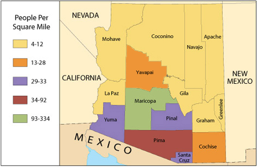
Figure 1.3.2, A map of Arizona and its counties color coded according to population. (“Arizona County Map,” National Atlas of the United States, 2004. http://nationalatlas.gov/printable/reference.html#list)
© BYU Independent Study
The next step is to create a graph depicting the number of counties in each of the population categories. I will use a computer map tool to make the graph. First, I will look at the colored map and count the number of counties for each population category; I then enter the totals in the computer program to create the graph you see below, Figure 1.3.3. I could make a similar graph using graph paper or by drawing a graph with straight lines on a blank piece of paper.
Now that the data is added to the map through the color-coding and the graph is made, we can use the map and the graph to answer some questions. Notice that the map makes it easy to answer certain questions and the graph makes it easy to answer other questions. In some cases you can use either the map or the graph to answer questions.
Try answering the following questions for your own practice:
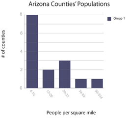
Figure 1.3.3
© BYU Independent Study
- Which area of Arizona has the heaviest population?
- Did you use the map or the graph to answer that question?
- The graph does not provide the information that we need to answer that question, but a quick look at the map shows us that the southern portion of the state has a much heavier population than the northern part of the state. Now try answering this question: are there more counties with a population of more than twelve people per square mile, or more counties with a population of twelve or fewer people per square mile?
You can solve this by using the map, but the graph is the most efficient way to see exactly how many counties fit into each population category. The graph shows that there are eight counties with a population of twelve or fewer people per square mile and it also shows us that there are seven counties with a population of more than twelve people per square mile. To get that information from the map you have to count each county individually. Since Arizona does not have many counties, this is not too difficult to do, but many states have a large number of counties and in those cases it is much easier to refer to a graph for this type of information.
Color Idaho Activity
Now it is your turn to make a population map and to create a graph. Use the data to add population information to the map of Idaho. You may print this map to color if you wish, or use the interactive Color Idaho activity which appears on the next page.
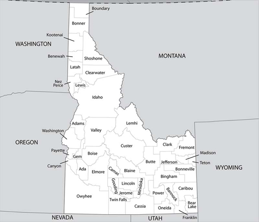
Figure 1.3.4, An outline map of Idaho and its counties, ready to be colored.
© BYU Independent Study
You can open a printable legend if you would like to mark the colors next to the names of the counties before color-coding the map.
| County | Population | County | Population |
|---|---|---|---|
|
Ada |
88–285 |
Gem |
22–50 |
|
Adams |
1–9 |
Gooding |
10–21 |
|
Bannock |
51–87 |
Idaho |
1–9 |
|
Bear Lake |
1–9 |
Jefferson |
10–21 |
|
Benewah |
1–9 |
Jerome |
1–9 |
|
Bingham |
10–21 |
Kootenai |
10–21 |
|
Blaine |
1–9 |
Latah |
22–50 |
|
Boise |
1–9 |
Lemhi |
1–9 |
|
Bonner |
51–87 |
Lewis |
1–9 |
|
Bonneville |
22–50 |
Lincoln |
1–9 |
|
Boundary |
10–21 |
Madison |
51–87 |
|
Butte |
1–9 |
Minidoka |
1–9 |
|
Camas |
1–9 |
Nez Perce |
22–50 |
|
Canyon |
88–285 |
Oneida |
1–9 |
|
Caribou |
1–9 |
Owyhee |
1–9 |
|
Cassia |
22–50 |
Payette |
22–50 |
|
Clark |
1–9 |
Power |
1–9 |
|
Clearwater |
1–9 |
Shoshone |
1–9 |
|
Custer |
1–9 |
Teton |
10–21 |
|
Elmore |
1–9 |
Twin Falls |
22–50 |
|
Franklin |
51–87 |
Valley |
1–9 |
|
Fremont |
1–9 |
Washington |
1–9 |
| Color | Population |
|---|---|
|
Red |
1–9 |
|
Yellow |
10–21 |
|
Green |
22–50 |
|
Purple |
51–87 |
|
Orange |
88–285 |
Color-code the counties on the map using the data and legend provided. Check the chart and legend above to find out the number of people per square mile and color the county accordingly. Once you have colored the entire map, click the check button to see what you got right. Once your map is right, print it or keep it open on screen so that you can use it to create your graph.
Color-coding activity with Idaho’s counties
© BYU Independent Study